NLP系列之文本分类

1前言

本篇博客主要是记录自然语言处理中的文本分类任务中常见的基础模型的使用及分析。Github上brightmart大佬已经整理出很完整的一套文本分类任务的基础模型及对应的模型代码实现。网上也有部分博客将brightmart写的模型实现步骤进行翻译整理出来了。本着尊重原创的原则，后面都列出了参考链接，在此也感谢参考链接上的作者。本文将对之前文本分类基础模型的博客和文献进行整理，此外再加上自己的一部分模型分析。毕竟还是需要有自己的东西在这里的，这样才能做到又学到了又进行思考了。

2文本分类任务

2.1 文本分类是自然语言处理中很基础的任务，是学习自然语言处理入门的很好的实际操作的任务，笔记当时就是从文本分类开始动手实践。文本分类的任务主要是把根据给出的文本(包括长文本，比如说资讯、新闻、文档等，也包括短文本，比如说评论，微博等)利用自然语言处理技术对文本进行归类整理，简单点说就是说给文本进行类别标注。
2.2 常见的文本分类模型有基于机器学习的分类方法和基于深度学习的分类方法。对于基于机器学习的分类方法，显然特征的提取和特征的选择过程将会对分类效果起到至关重要的作用。在文本的特征提取上，基于词级层面的TF-IDF特征，n-gram特征，主题词和关键词特征。基于句子级别的有句式，句子长度等特征。基于语义层面的特征可以使用word2vec预训练语料库得到词向量，使用词向量合理的构造出文本的词向量作为文本的语义特征。对于基于深度学习的文本分类方法，显然模型的结构和模型的参数将会对分类效果起到至关作用。在模型结构上常用的基础的神经网络模型有CNN，RNN，GRU，Attention机制，Dropout等。在模型参数的调节上，一方面需要设定好模型的参数学习率，另一位方面需要根据模型的使用特点和要分析的文本内容进行调节。
说明： 本文通过介绍brightmart在基础神经网络在文本分类上的实验来进行相关的模型介绍和模型分析，该实验主要是在2017年知乎看山杯的一道竞赛题，竞赛内容是对知乎上的问题进行分类，当然此次任务属性文本分类中多标签分类，属于文本分类的范畴。
2.3各个基模型的实验结果
brightmart使用以下的基础模型在上述数据集上进行了大量实验，实验结果如下。以下很多模型比较基础，都是非常经典的模型，作为实验的基准模型BaseLine是非常合适的。如果想继续提升实验结果，可能就需要根据数据的特征进行模型的改进或者模型的集成工作了。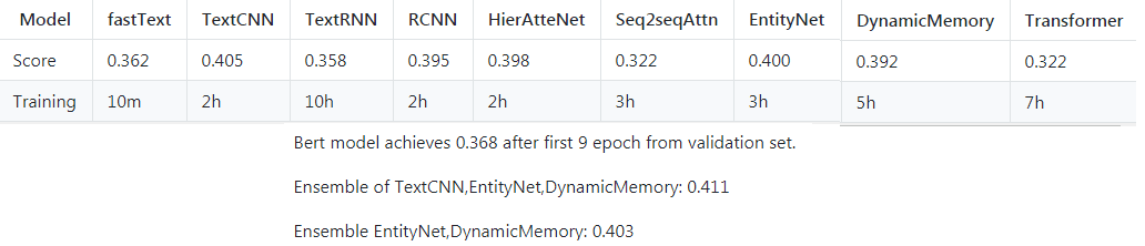
实验对比图

3基础文本分类模型的介绍及分析

本部分主要对基础的文本分类进行介绍，主要分为模型结构的论文来源介绍，模型结构，模型的实现步骤，代码的主要实现(也是来自brightmart的项目)和最后关于模型的分析。

3.1FastText

3.1.1论文来源
《Bag of Tricks for Efficient Text Classification》
3.1.2模型结构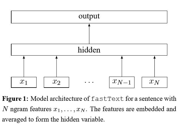
fasttext 3.1.3模型的实现步骤

从模型的结构可以看出，FastText的模型的实现步骤为：
1.embedding–>2.average–>3.linear classifier(没有经过激活函数)-> SoftMax分类

3.1.4模型的关键实现代码

# 其中None表示你的batch_size大小
#1.get emebedding of words in the sentence
sentence_embeddings = tf.nn.embedding_lookup(self.Embedding,self.sentence)  # [None,self.sentence_len,self.embed_size]
#2.average vectors, to get representation of the sentence
self.sentence_embeddings = tf.reduce_mean(sentence_embeddings, axis=1)  # [None,self.embed_size]
#3.linear classifier layer
logits = tf.matmul(self.sentence_embeddings, self.W) + self.b #[None, self.label_size]==tf.matmul([None,self.embed_size],[self.embed_size,self.label_size])

3.1.5模型的分析

FastText的模型结构相对是比较简单的，是一个有监督的训练模型。我们知道FastText训练不仅可以得到分类的效果，如果语料充足的话，可以训练得到词向量。
1. FastText模型结构简单，因为最后对文本的分类都是直接经过线性层来进行分类的，可以说是完成线性的，最后是没有经过激活函数。因此句子结构比较简单的文本分类任务来说，FastText是可以进行的。对于复杂的分类任务，比如说情感分类等，由于网络模型需要学习到语句的语义，语序等特征，显然对于简单的线性层分类是不足的，因此还是需要引入复杂的非线性结构层。正因为模型结构简单，模型训练速度是相对较快的。
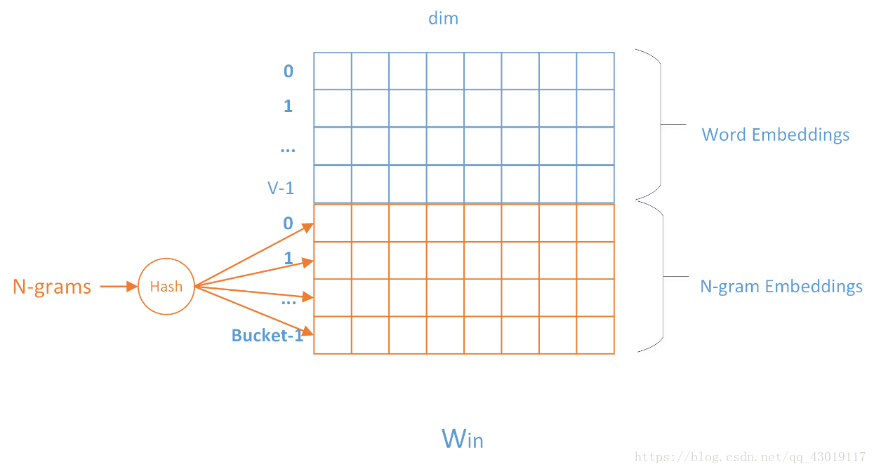
2. FastText引入了N gram特征。从FastText前面的模型结构中，第二层计算的是词向量的平均值，此步骤将会忽略掉文本的词序特征。显然对于文本的分类任务中，这将会损失掉词序特征的。因此，在FastText词向量中引入了N gram的词向量。具体做法是，在N gram也当做一个词，因此也对应着一个词向量，在第二层计算词向量的均值的时候，也需要把N gram对应的词向量也加进来进行计算平均值。通过训练分类模型，这样可以得到词向量和N gram对应的词向量。期间也会存在一个问题，N gram的量其实远比word大的多。因此FastText采用Hash桶的方式，把所有的N gram都哈希到buckets个桶中，哈希到同一个桶的所有n-gram共享一个embedding vector。这点可以联想到，在处理UNK的词向量的时候，也可以使用类似的思想进行词向量的设置。

3.2TextCNN

3.2.1论文来源
《Convolutional Neural Networks for Sentence Classification》
3.2.2模型结构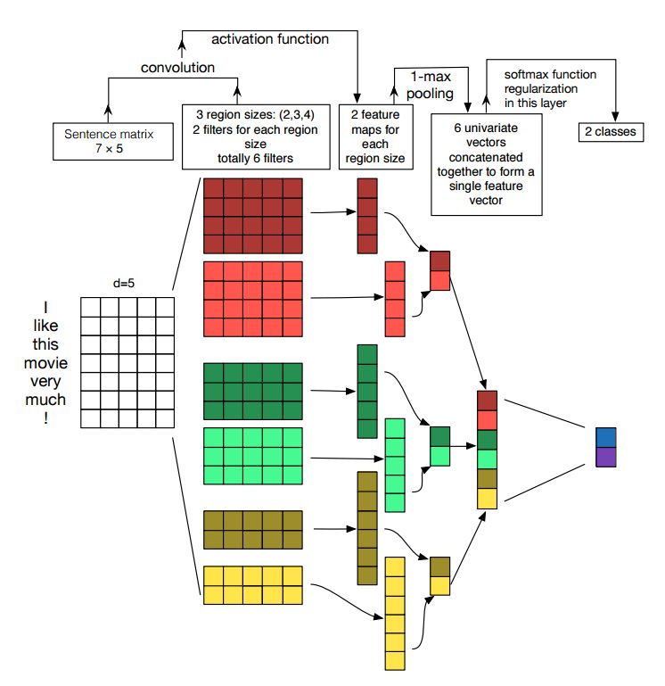
词向量图 3.2.3模型的实现步骤

从模型的结构可以看出，TextCNN的模型的实现步骤为：
1.embedding—>2.conv—>3.max pooling—>4.fully connected layer——–>5.softmax

3.2.4模型的关键实现代码

# 1.=====>get emebedding of words in the sentence
self.embedded_words = tf.nn.embedding_lookup(self.Embedding,self.input_x)#[None,sentence_length,embed_size]
self.sentence_embeddings_expanded=tf.expand_dims(self.embedded_words,-1) #[None,sentence_length,embed_size,1). expand dimension so meet input requirement of 2d-conv
# 2.=====>loop each filter size. for each filter, do:convolution-pooling layer(a.create filters,b.conv,c.apply nolinearity,d.max-pooling)--->
# you can use:tf.nn.conv2d;tf.nn.relu;tf.nn.max_pool; feature shape is 4-d. feature is a new variable
#if self.use_mulitple_layer_cnn: # this may take 50G memory.
        #    print("use multiple layer CNN")
        #    h=self.cnn_multiple_layers()
        #else: # this take small memory, less than 2G memory.
print("use single layer CNN")
h=self.cnn_single_layer()
#5. logits(use linear layer)and predictions(argmax)
with tf.name_scope("output"):
    logits = tf.matmul(h,self.W_projection) + self.b_projection  #shape:[None, self.num_classes]==tf.matmul([None,self.embed_size],[self.embed_size,self.num_classes])

3.2.5模型的分析
笔者之前详细介绍过一篇TextCNN实现的博客，可以查看卷积神经网络(TextCNN)在句子分类上的实现

深度学习与机器学习的最重要的不同之处便是：深度学习使用神经网络代替人工的进行特征的抽取。所以，最终模型的效果的好坏，其实是和神经网络的特征抽取的能力强弱相关。在文本处理上，特征抽取能力主要有句法特征提取能力；语义特征提取能力；长距离特征捕获能力；任务综合特征抽取能力。上面四个角度是从NLP的特征抽取器能力强弱角度来评判的，另外再加入并行计算能力及运行效率，这是从是否方便大规模实用化的角度来看的。
1. TextCNN神经网络主要以CNN网络对文本信息进行特征的抽取，在图像的处理上，CNN的特征抽取能力是非常强的。我们把词向量的维度和文本的长度当成另一个维度是可以构成一个矩阵的，于是，CNN便可以在文本进行卷积核的计算(文本的特征抽取)。此时，卷积核的大小就相当于N gram的特征了。
2. TextCNN中的实现步骤中是有max pooling的一步的。具体过程是多个卷积核对文本进行滑动获取语义特征，而CNN中的卷积核是能保留特征之间的相对位置的，因为卷积核是滑动的，从左至右滑动，因此捕获到的特征也是如此顺序排列，所以它在结构上已经记录了相对位置信息了。但是卷积层后面立即接上Pooling层的话，Max Pooling的操作逻辑是：从一个卷积核获得的特征向量里只选中并保留最强的那一个特征，所以到了Pooling层，位置信息就被损失掉了(信息损失)。因此在对应需要捕获文本的词序信息特征时，pooling层应该需要添加上位置信息。

3.3TextRNN/LSTM

3.3.1模型结构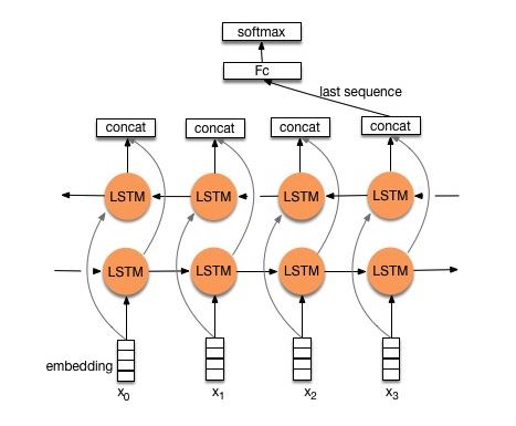
词向量图 3.3.2模型的步骤

从模型的结构可以看出，TextRNN/LSTM的模型的实现步骤为：
1.embedding—>2.bi-directional lstm—>3.concat output—>4.average/last output—–>5.softmax layer

3.3.3模型的关键实现代码

#1.get emebedding of words in the sentence
self.embedded_words = tf.nn.embedding_lookup(self.Embedding,self.input_x) #shape:[None,sentence_length,embed_size]
#2. Bi-lstm layer
# define lstm cess:get lstm cell output
lstm_fw_cell=rnn.BasicLSTMCell(self.hidden_size) #forward direction cell
lstm_bw_cell=rnn.BasicLSTMCell(self.hidden_size) #backward direction cell
if self.dropout_keep_prob is not None:
    lstm_fw_cell=rnn.DropoutWrapper(lstm_fw_cell,output_keep_prob=self.dropout_keep_prob)
    lstm_bw_cell=rnn.DropoutWrapper(lstm_bw_cell,output_keep_prob=self.dropout_keep_prob)
# bidirectional_dynamic_rnn: input: [batch_size, max_time, input_size]
#                            output: A tuple (outputs, output_states)
#                                    where:outputs: A tuple (output_fw, output_bw) containing the forward and the backward rnn output `Tensor`.
outputs,_=tf.nn.bidirectional_dynamic_rnn(lstm_fw_cell,lstm_bw_cell,self.embedded_words,dtype=tf.float32) #[batch_size,sequence_length,hidden_size] #creates a dynamic bidirectional recurrent neural network
print("outputs:===>",outputs) #outputs:(<tf.Tensor 'bidirectional_rnn/fw/fw/transpose:0' shape=(?, 5, 100) dtype=float32>, <tf.Tensor 'ReverseV2:0' shape=(?, 5, 100) dtype=float32>))
#3. concat output
output_rnn=tf.concat(outputs,axis=2) #[batch_size,sequence_length,hidden_size*2]
#4.1 average
#self.output_rnn_last=tf.reduce_mean(output_rnn,axis=1) #[batch_size,hidden_size*2]
#4.2 last output
self.output_rnn_last=output_rnn[:,-1,:] ##[batch_size,hidden_size*2] #TODO
print("output_rnn_last:", self.output_rnn_last) # <tf.Tensor 'strided_slice:0' shape=(?, 200) dtype=float32>
#5. logits(use linear layer)
with tf.name_scope("output"): #inputs: A `Tensor` of shape `[batch_size, dim]`.  The forward activations of the input network.
    logits = tf.matmul(self.output_rnn_last, self.W_projection) + self.b_projection  # [batch_size,num_classes]

3.3.4模型的分析

1. RNN是典型的序列模型结构，它是线性序列结构，它不断从前往后收集输入信息，但这种线性序列结构在反向传播的时候存在优化困难问题，因为反向传播路径太长，容易导致严重的梯度消失或梯度爆炸问题。为了解决这个问题，引入了LSTM和GRU模型，通过增加中间状态信息直接向后传播，由原来RNN的迭代乘法结构变为后面的加法结构，以此缓解梯度消失问题。于是上面是有LSTM或GRU来代替RNN。
2. RNN的线性序列结构，让RNN能很好的对不定长文本的输入进行接纳，将文本序列当做随着时间变换的序列状态，很好的接纳文本的从前向后的输入。在LSTM中引入门控制机制，从而使该序列模型能存储之前网络的特征，这对于捕获长距离特征非常有效。所以RNN特别适合NLP这种线形序列应用场景，这是RNN为何在NLP界如此流行的根本原因。
3. 因为RNN的序列结构，t时刻的状态是依赖t-1时刻的网络状态的，这对于网络大规模的并行进行是很不友好的。也就是说RNN的高效并行计算能力是比较差的。当然可以对RNN结构进行一定程度上的改进，使之拥有一定程度的并行能力。

3.4RCNN

3.4.1论文来源
《Recurrent Convolutional Neural Network for Text Classification》
3.4.2模型结构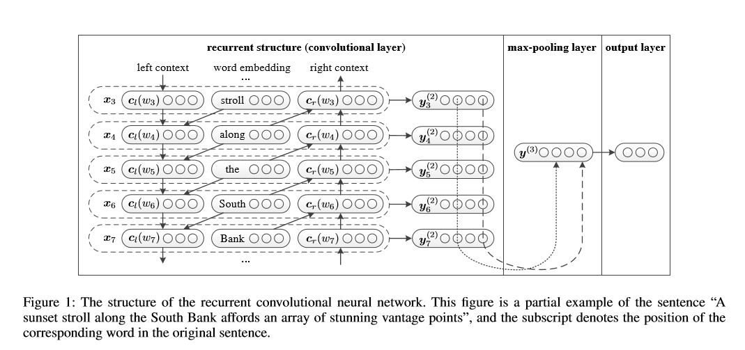
词向量图 3.4.3模型的步骤

从模型的结构可以看出，RCNN的模型的实现步骤为：
1.emebedding–>2.recurrent structure (convolutional layer)—>3.max pooling—>4.fully connected layer+softmax

3.4.4模型的关键实现代码

#1.get emebedding of words in the sentence
self.embedded_words = tf.nn.embedding_lookup(self.Embedding,self.input_x) #shape:[None,sentence_length,embed_size]
#2. Bi-lstm layer
output_conv=self.conv_layer_with_recurrent_structure() #shape:[None,sentence_length,embed_size*3]
#3. max pooling
#print("output_conv:",output_conv) #(3, 5, 8, 100)
output_pooling=tf.reduce_max(output_conv,axis=1) #shape:[None,embed_size*3]
#print("output_pooling:",output_pooling) #(3, 8, 100)
#4. logits(use linear layer)
with tf.name_scope("dropout"):
    h_drop=tf.nn.dropout(output_pooling,keep_prob=self.dropout_keep_prob) #[None,num_filters_total]

with tf.name_scope("output"): #inputs: A `Tensor` of shape `[batch_size, dim]`.  The forward activations of the input network.
    logits = tf.matmul(h_drop, self.W_projection) + self.b_projection  # [batch_size,num_classes]
def conv_layer_with_recurrent_structure(self):
        """
        input:self.embedded_words:[None,sentence_length,embed_size]
        :return: shape:[None,sentence_length,embed_size*3]
        """
        #1. get splitted list of word embeddings
        embedded_words_split=tf.split(self.embedded_words,self.sequence_length,axis=1) #sentence_length个[None,1,embed_size]
        embedded_words_squeezed=[tf.squeeze(x,axis=1) for x in embedded_words_split]#sentence_length个[None,embed_size]
        embedding_previous=self.left_side_first_word
        context_left_previous=tf.zeros((self.batch_size,self.embed_size))
        #2. get list of context left
        context_left_list=[]
        for i,current_embedding_word in enumerate(embedded_words_squeezed):#sentence_length个[None,embed_size]
            context_left=self.get_context_left(context_left_previous, embedding_previous) #[None,embed_size]
            context_left_list.append(context_left) #append result to list
            embedding_previous=current_embedding_word #assign embedding_previous
            context_left_previous=context_left #assign context_left_previous
        #3. get context right
        embedded_words_squeezed2=copy.copy(embedded_words_squeezed)
        embedded_words_squeezed2.reverse()
        embedding_afterward=self.right_side_last_word
        context_right_afterward = tf.zeros((self.batch_size, self.embed_size))
        context_right_list=[]
        for j,current_embedding_word in enumerate(embedded_words_squeezed2):
            context_right=self.get_context_right(context_right_afterward,embedding_afterward)
            context_right_list.append(context_right)
            embedding_afterward=current_embedding_word
            context_right_afterward=context_right
        #4.ensemble left,embedding,right to output
        output_list=[]
        for index,current_embedding_word in enumerate(embedded_words_squeezed):
            representation=tf.concat([context_left_list[index],current_embedding_word,context_right_list[index]],axis=1)
            #print(i,"representation:",representation)
            output_list.append(representation) #shape:sentence_length个[None,embed_size*3]
        #5. stack list to a tensor
        #print("output_list:",output_list) #(3, 5, 8, 100)
        output=tf.stack(output_list,axis=1) #shape:[None,sentence_length,embed_size*3]
        #print("output:",output)
        return output

3.4.5模型的分析

1. 从RCNN的模型结构来看，做出重大改变的是词向量的表示，以往的词向量的表示即是简单的一个词的[word embedding],而RCNN中的表示为[left context; word embedding, right context],从词向量中引入上下文语境。具体的left context=activation(pre left contextWl+ pre word embedding Ww)。right context则反过来为之。
2. RCNN比TextRNN实验的效果是好的，改进后的word embedding起到了很重要的作用。一个词用一个词向量来表示这其实是有一定的局限性的，当遇到一词多意的时候，使用一个词向量来表示一个词，此时就显得不那么恰当了，因为使用一个词向量来表示，这相当于对所有的词义进行了平均获得的。我们可以理解这种一词一个向量的表示为静态词向量。而RCNN中则在原词向量上添加左右context，这相当于引入了词的语境，可以理解为对原单个词向量进行了一定程度上的调整，让一词多义的表示成为可能。

3.5Hierarchical Attention Network

3.5.1论文来源
《Hierarchical Attention Networks for Document Classification》
3.5.2模型结构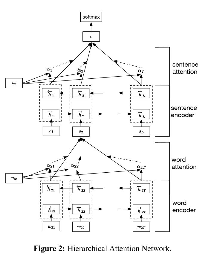
词向量图 3.5.3模型的步骤

从模型的结构可以看出，HAN的模型的实现步骤为：
1.emebedding–>2.word encoder(bi-directional GRU)—>3.word Attention—>4.Sentence Encoder(bi-directional GRU)—>5.Sentence Attetion—>6.fC+Softmax

3.5.4模型的关键实现代码

# 1.1 embedding of words
input_x = tf.split(self.input_x, self.num_sentences,axis=1)  # a list. length:num_sentences.each element is:[None,self.sequence_length/num_sentences]
input_x = tf.stack(input_x, axis=1)  # shape:[None,self.num_sentences,self.sequence_length/num_sentences]
self.embedded_words = tf.nn.embedding_lookup(self.Embedding,input_x)  # [None,num_sentences,sentence_length,embed_size]
embedded_words_reshaped = tf.reshape(self.embedded_words, shape=[-1, self.sequence_length,self.embed_size])  # [batch_size*num_sentences,sentence_length,embed_size]
# 1.2 forward gru
hidden_state_forward_list = self.gru_forward_word_level(embedded_words_reshaped)  # a list,length is sentence_length, each element is [batch_size*num_sentences,hidden_size]
# 1.3 backward gru
hidden_state_backward_list = self.gru_backward_word_level(embedded_words_reshaped)  # a list,length is sentence_length, each element is [batch_size*num_sentences,hidden_size]
# 1.4 concat forward hidden state and backward hidden state. hidden_state: a list.len:sentence_length,element:[batch_size*num_sentences,hidden_size*2]
self.hidden_state = [tf.concat([h_forward, h_backward], axis=1) for h_forward, h_backward in
                     zip(hidden_state_forward_list, hidden_state_backward_list)]  # hidden_state:list,len:sentence_length,element:[batch_size*num_sentences,hidden_size*2]

# 2.Word Attention
# for each sentence.
sentence_representation = self.attention_word_level(self.hidden_state)  # output:[batch_size*num_sentences,hidden_size*2]
sentence_representation = tf.reshape(sentence_representation, shape=[-1, self.num_sentences, self.hidden_size * 2])  # shape:[batch_size,num_sentences,hidden_size*2]
#with tf.name_scope("dropout"):#TODO
#    sentence_representation = tf.nn.dropout(sentence_representation,keep_prob=self.dropout_keep_prob)  # shape:[None,hidden_size*4]

# 3.Sentence Encoder
# 3.1) forward gru for sentence
hidden_state_forward_sentences = self.gru_forward_sentence_level(sentence_representation)  # a list.length is sentence_length, each element is [None,hidden_size]
# 3.2) backward gru for sentence
hidden_state_backward_sentences = self.gru_backward_sentence_level(sentence_representation)  # a list,length is sentence_length, each element is [None,hidden_size]
# 3.3) concat forward hidden state and backward hidden state
# below hidden_state_sentence is a list,len:sentence_length,element:[None,hidden_size*2]
self.hidden_state_sentence = [tf.concat([h_forward, h_backward], axis=1) for h_forward, h_backward in zip(hidden_state_forward_sentences, hidden_state_backward_sentences)]

# 4.Sentence Attention
document_representation = self.attention_sentence_level(self.hidden_state_sentence)  # shape:[None,hidden_size*4]
with tf.name_scope("dropout"):
    self.h_drop = tf.nn.dropout(document_representation,keep_prob=self.dropout_keep_prob)  # shape:[None,hidden_size*4]
# 5. logits(use linear layer)and predictions(argmax)
with tf.name_scope("output"):
    logits = tf.matmul(self.h_drop, self.W_projection) + self.b_projection  # shape:[None,self.num_classes]==tf.matmul([None,hidden_size*2],[hidden_size*2,self.num_classes])
return logits

3.5.5模型的分析

1. Hierarchical Attention Network(HAN)分层对文本进行构建模型(Encoder)，此外在每层加上了两个Attention层，分别表示对文本中的按错和句子的重要性进行建模。HAN比较适用于长文本的分类，长文本包括多个句子，句子中包括多个词，适用于对文本的分层建模。首先，HAN考虑到文本的层次结构：词构成句，句子构成文档。因此，对文本的建模时也针对这两部分。因为一个句子中每个词对分类的结果影响的不一样，一个句子对文本分类的结果影响也不一样。所以，引入Attention机制，这样每个词，每个句子的对分类的结果的影响将不会一样。具体计算的公式如下：

3.6Transformer

3.6.1论文来源
《Attention Is All You Need》
3.6.2模型结构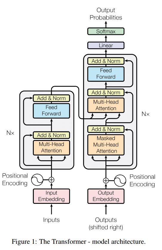
transformer 3.6.3模型的步骤

从模型的结构可以看出，Transformer的模型的实现步骤为：
1.word embedding&position embedding–>2.Encoder(2.1multi head self attention->2.2LayerNorm->2.3position wise fully connected feed forward network->2.4LayerNorm)—>3.linear classifie

3.6.4模型的关键实现代码

input_x_embeded = tf.nn.embedding_lookup(self.Embedding,self.input_x)  #[None,sequence_length, embed_size]
input_x_embeded=tf.multiply(input_x_embeded,tf.sqrt(tf.cast(self.d_model,dtype=tf.float32)))
input_mask=tf.get_variable("input_mask",[self.sequence_length,1],initializer=self.initializer)
input_x_embeded=tf.add(input_x_embeded,input_mask) #[None,sequence_length,embed_size].position embedding.

# 2. encoder
encoder_class=Encoder(self.d_model,self.d_k,self.d_v,self.sequence_length,self.h,self.batch_size,self.num_layer,input_x_embeded,input_x_embeded,dropout_keep_prob=self.dropout_keep_prob,use_residual_conn=self.use_residual_conn)
Q_encoded,K_encoded = encoder_class.encoder_fn() #K_v_encoder

Q_encoded=tf.reshape(Q_encoded,shape=(self.batch_size,-1)) #[batch_size,sequence_length*d_model]
with tf.variable_scope("output"):
    logits = tf.matmul(Q_encoded, self.W_projection) + self.b_projection #logits shape:[batch_size*decoder_sent_length,self.num_classes]
print("logits:",logits)
return logits
def encoder_single_layer(self,Q,K_s,layer_index):
    """
    singel layer for encoder.each layers has two sub-layers:
    the first is multi-head self-attention mechanism; the second is position-wise fully connected feed-forward network.
    for each sublayer. use LayerNorm(x+Sublayer(x)). input and output of last dimension: d_model
    :param Q: shape should be:       [batch_size*sequence_length,d_model]
    :param K_s: shape should be:     [batch_size*sequence_length,d_model]
    :return:output: shape should be:[batch_size*sequence_length,d_model]
    """
    #1.1 the first is multi-head self-attention mechanism
    multi_head_attention_output=self.sub_layer_multi_head_attention(layer_index,Q,K_s,self.type,mask=self.mask,dropout_keep_prob=self.dropout_keep_prob) #[batch_size,sequence_length,d_model]
    #1.2 use LayerNorm(x+Sublayer(x)). all dimension=512.
    multi_head_attention_output=self.sub_layer_layer_norm_residual_connection(K_s ,multi_head_attention_output,layer_index,'encoder_multi_head_attention',dropout_keep_prob=self.dropout_keep_prob,use_residual_conn=self.use_residual_conn)

    #2.1 the second is position-wise fully connected feed-forward network.
    postion_wise_feed_forward_output=self.sub_layer_postion_wise_feed_forward(multi_head_attention_output,layer_index,self.type)
    #2.2 use LayerNorm(x+Sublayer(x)). all dimension=512.
    postion_wise_feed_forward_output= self.sub_layer_layer_norm_residual_connection(multi_head_attention_output,postion_wise_feed_forward_output,layer_index,'encoder_postion_wise_ff',dropout_keep_prob=self.dropout_keep_prob)
    return  postion_wise_feed_forward_output,postion_wise_feed_forward_output

3.6.5模型的分析

1. 论文《Attention is all you need》中的Transformer指的是完整的Encoder-Decoder框架，而对于此项文本分类来说，Transformer是其中对应的Encoder，而一个Encoder模块(Block)包含着多个子模块(包括Multi-head self attention，Skip connection，LayerNorm，Feed Forward)，如下：2. 对于Transformer来说，需要明确加入位置编码学习position Embedding.因为对于self Attention来说，它让当前输入单词和句子中任意单词进行相似计算，然后归一化计算出句子中各个单词对应的权重，再利用权重与各个单词对应的变换后V值相乘累加，得出集中后的embedding向量，此间是损失掉了位置信息的。因此，为了引入位置信息编码，Transformer对每个单词一个Position embedding，将单词embedding和单词对应的position embedding加起来形成单词的输入embedding。
3.Transformer中的self Attention对文本的长距离依赖特征的提取有很强的能力，因为它让当前输入单词和句子中任意单词进行相似计算，它是直接进行的长距离依赖特征的获取的，不像RNN需要通过隐层节点序列往后传，也不像CNN需要通过增加网络深度来捕获远距离特征。此外，对应模型训练时的并行计算能力，Transformer也有先天的优势，它不像RNN需要依赖前一刻的特征量。
4. 张俊林大佬在【6】中提到过，在Transformer中的Block中不仅仅multi-head attention在发生作用，而是几乎所有构件都在共同发挥作用，是一个小小的系统工程。例如Skip connection，LayerNorm等也是发挥了作用的。对于Transformer来说，Multi-head attention的head数量严重影响NLP任务中Long-range特征捕获能力：结论是head越多越有利于捕获long-range特征。

4总结

1.对于一个人工智能领域的问题的解决，不管是使用深度学习的神经网络还是使用机器学习的人工特征提取，效果的好坏主要是和特征器的提取能力挂钩的。机器学习使用人工来做特征提取器，对于问题的解决原因，可解释性强。而深度学习的数据网络结构使用线性的和非线性的神经元节点相结合比较抽象的作为一个特征提取器。
在文本处理上，特征抽取能力主要包括有有句法特征提取能力；语义特征提取能力；长距离特征捕获能力；任务综合特征抽取能力。上面四个角度是从NLP的特征抽取器能力强弱角度来评判的，另外再加入并行计算能力及运行效率，这是从是否方便大规模实用化的角度来看的。
而对于各个领域的的问题的解决，新浪微博AI Lab资深算法专家张俊林博士大佬说过一句话：一个特征抽取器是否适配问题领域的特点，有时候决定了它的成败，而很多模型改进的方向，其实就是改造得使得它更匹配领域问题的特性。
2.对于输出空间巨大的大规模文本分类问题。事实上，对于文本的生成问题(对于其中一个单词的生成)，可以看做是输出空间巨大的大规模文本的文本分类问题。在Word2vec中，解决的方法是使用层次softmax的方法，首先对分类的标签进行哈夫曼树的构建，每个分类标签对应着一个哈夫曼码，位于哈夫曼树的叶子结点，其中每个分支表示通往每个路径的概率。此外，word2vec中也提出negative sampling的方式，因此可以考虑使用 negative sampling的方式来解决此类问题，对标签的样本重新进行构建二分类，首先(x,y)表示正确的样本为正样本，然后根据分类标签的概率分布进行采样德奥(x,y‘)作为负样本，重构成二分类问题。常在Seq2Seq的生成中，采用【8】Sampled Softmax、Adaptive softmax等方式来缓解输出空间巨大的大规模文本分类。
3.对于标签存在一定关联的情况下的文本分类。我们常常做的文本分类是使用一对一或者一对多方法的方法进行分类器的训练，例如SVM或者NB等。如果标签也存在一点的联系，如标签类目树，或者单个标签与单个标签存在相关性等。对于单个标签与单个标签存在相关性，目前有人将此类多标签问题当做序列生成问题来解决，效果性能得到了很大的改进,对应的论文有SGM: Sequence Generation Model for Multi-Label Classification.还有对标签层次化问题进行了研究的相关论文A Study of multilabel text classification and the effect of label hierarchy
4.基于深度学习技术的文本分类技术比起传统的文本分类模型(LR，SVM 等)的优势。首先，免去了人工的提取文本特征，它可以自动的获取基础特征并组合为高级的特征，训练模型获得文本特征与目标分类之间的关系，省去了使用TF-IDF等提取句子的关键词构建特征工程的过程，实现端到端。其次，相比传统的N-gram模型而言，深度学习中可以更好的利用词序的特征，CNN的文本分类模型中的filter的size的大小可以当做是一种类似于N-gram的方式，而RNN（LSTM）则可以利用更长的词序，配合Attention机制则可以通过加权矩阵体现句子中的核心词汇部位。最后，随着样本的增加和网络深度的增加，深度学习的分类精度会更高。

5参考链接

【1】brightmart/text_classification
【2】The Annotated Transformer
【3】fastText、TextCNN、TextRNN…这套NLP文本分类深度学习方法库供你选择
【4】word2vec、glove和 fasttext 的比较
【5】从Word Embedding到Bert模型——自然语言处理预训练技术发展史
【6】放弃幻想，全面拥抱Transformer：自然语言处理三大特征抽取器（CNN/RNN/TF）比较
【7】《BERT: Pre-training of Deep Bidirectional Transformers for Language Understanding》
【8】Sampled Softmax 论文笔记：On Using Very Large Target Vocabulary for Neural Machine Translation